Joining tables in the Persistent Staging Area

In this blog post, I would like to share a pattern for joining tables in the staging layer of the data solution – specifically in the Persistent Staging Area (PSA). It is something that comes up regularly, and can arguably best be described as somewhat of an ‘anti pattern’.

Ideally, you would try to avoid joining tables in the staging layer where possible. This is because this pattern involves bringing forward complexities and considerations that are usually best addressed in the integration layer of the data solution.

However, depending on your scenario, it could also be a very practical solution that avoids downstream complexities. We should not entirely discard this pattern either.

When joining data in the staging layer, we should always do so using the PSA tables. The PSA contains a transactional, historised, record of all data transactions that have ever been presented to the data solution. It is the transaction log containing all raw data events, and is invaluable for a truly flexible data solution.

This full history of original data changes is exactly what is needed to correctly join the different data sets together. By contrast, the staging (or landing) area that is also part of the staging layer is transient, and is therefore not fit for purpose simply because the tables might be empty at any given moment.

There are some exceptions to this, for example if you store full data snapshots across all tables each processing run in the staging/landing area. But, this is not a common pattern because of scalability concerns. And, the PSA approach always works, and is not impacted by any data loading dependencies (but is more complicated).

In all cases, it is recommended to refrain from adding any business logic that changes the nature of the data; no destructive transformations. After all, the goal of the staging layer is to correctly ingest and historise ‘raw’ data (transactions) without passing judgement on it – that is done later in the data solution.

The sweet spot for this pattern is when you want to associate various columns to a certain Core Business Concept (CBC) e.g. a ‘Hub’ table in Data Vault, but the tables in question do not contain the business key you need for this CBC. Or, you just want all related columns in a single wider table.

In other words, the business key and context columns you need are separated by a few tables that contain Foreign Key references.

So how does this work?

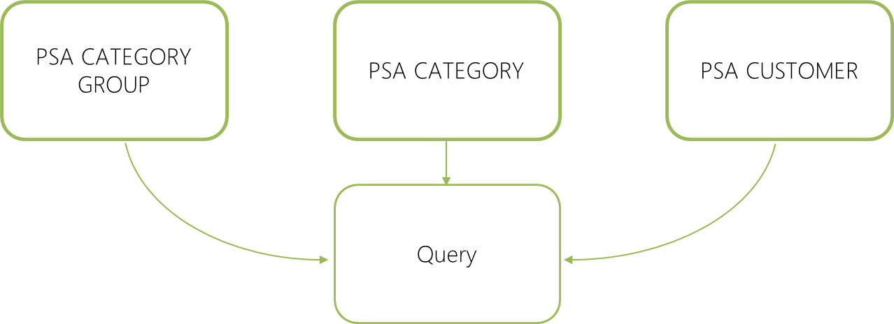
Customer, Category, Category Group

Imagine the following scenario:

• A customer is assigned a category, and
• A category may contain many customers (or none), and has a name
• Every category belongs to a category group, a category group also has a name property and can cover many categories

Your ideal query would contain customer information including the corresponding category name and category group name.

In this example, you might want to define the category name and category group name as direct descriptive properties of the ‘Customer’ CBC. It could be a classification of the customer, and it may not be required to define this as a separate CBC and corresponding relationship.

We can join the involved PSA tables together to provide this as a single result set for easy downstream processing.

The trick for this pattern, is to acknowledge that all three tables may incur data changes over time, and at different frequencies. Sometimes, the category group name value may be updated. This would not, however, directly change anything in the category or customer tables. The data change would only apply to the category group table in this case, because the Foreign Key value in the referenced table is not updated.

But it does affect the result when all three tables are joined together.

Each involved table may experience data changes being inserted at different intervals, and the join query represents the combined changes that happen across all involved tables.

In this particular example though, we are only interested in changes from the customer (table) perspective. We don’t really need to know about any categories or category groups that are not referenced by any customer. After all, the goal is to only add the customer context to the customer CBC.

This consideration drives the approach for joining the tables, as illustrated in the diagram below.

To display the combined changes across all tables, we can query them by starting from each table individually and joining in the other ones. This means running three separate queries in this example, each selecting the data from its unique perspective.

The combination (union) of these three queries will provide the final result.

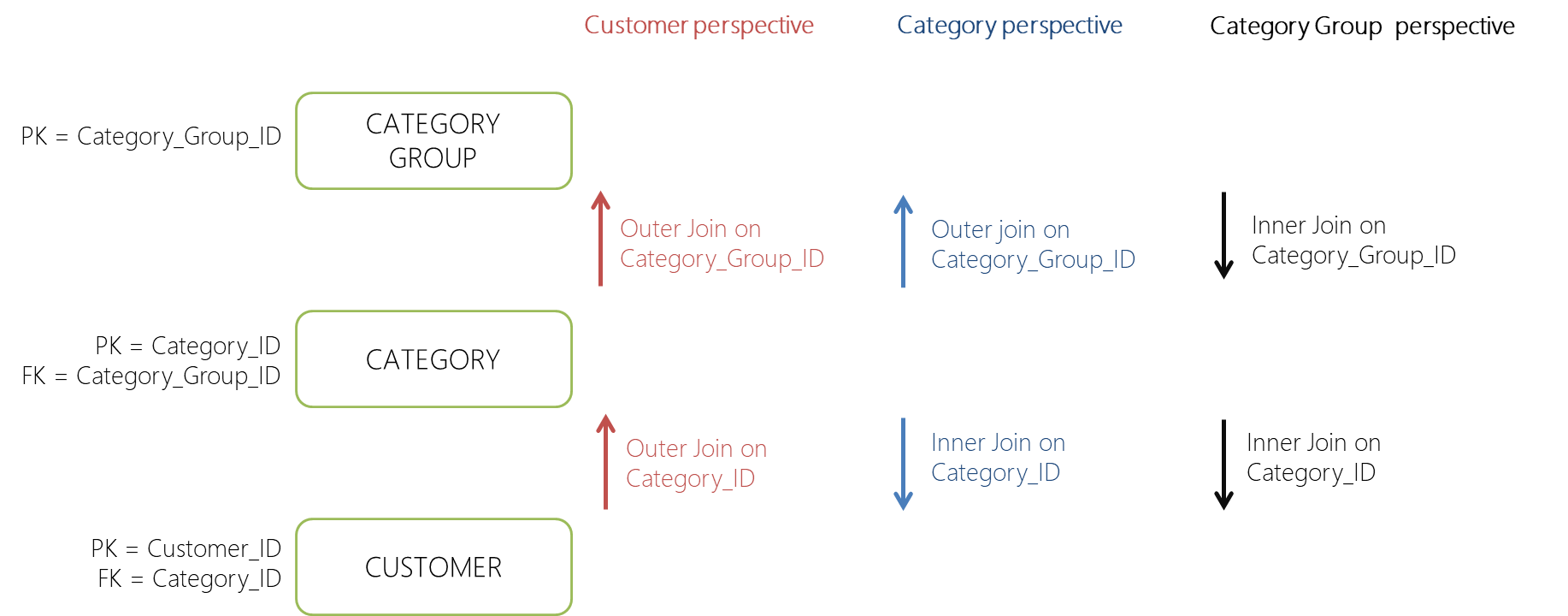
Using the customer table as starting point, the category can be outer-joined directly from the customer table. After this, the category group can be outer-joined via the category table. Both joins are outer joins because we don’t want to ‘lose’ customer records because the category or category group is not (yet) available. This should not be possible according to the original Entity-Relationship diagram, but we also have to consider the data loading frequencies. Some data may not yet be loaded.

When starting from the perspective of the category table, the customer table can be inner-joined. This is because we are only interested in categories that are associated to customers. The join to the category group is an outer join again, since we don’t want to miss out on customer/category records that do not happen to have a category group yet.

Lastly, the category group starting point inner-joins to the other table. Only categories/customers that are referenced are of interest.

Each of these queries provide a subset of changes that are relevant for the full set. I have added two examples of how to implement this as downloadable SQL code near the end of this post.

How to join in the PSA

When joining time-variant (historised) tables, such as is the case for the PSA, you must take the ‘time’ element into account when joining data. Each PSA record represents a version of the record (key) as it was at a point in time, ordered by the inscription timestamp (moment of arrival).

But, the inscription timestamp is a technical value, managed by the data solution to secure full auditability on when data became known to the solution.

It is conceptually not a great candidate to join data with.

For more details on this, please read the various posts on (bi)temporality in the data solution.

In short, the moment that data became known to the data solution is often relevant for joining the matching category or category group to the customer, as it was back in time. The data may contain its own validity periods, which are very likely the ones expected by the data consumers.

And this is where the challenges are when joining tables in the PSA.

Because you must join the tables using a suitable timeline, you effectively bring-forward the complexities that are otherwise addressed in the integration layer – when switching over to delivering data according to the (standardised) reporting timeline referred to as the state timeline.

Not only is this timeline not ready yet, it also potentially exposes the solution to data quality issues (e.g. overlaps, gaps, duplications) caused by questionable date/time values. A correct timeline for data delivery has been uniquified. In the example, this is represented by using the term ‘date_key’ as opposed to the effective date directly.

These challenges are not insurmountable, but must be adequately considered and investigated.

Consider the example below, which covers two out of the three tables used in the earlier example (for brevity). The top result set shows the data in the ‘customer’ table. The middle data set represents the data in the ‘category’ table, and the bottom result set contains the combined changes across both tables after joining.

For joining the tables in their correct point in time, the ‘effective date’ column has been used. For this to work, a date range can be created using this column, and applied to create the correct point-in-time join.

In the result you can see all three customer records being represented. This is expected, because the category is outer-joined.

The first two records from the category table are not found in the final result set, however. There was no customer associated with this category at that point in time, so the inner join removed this record.

The final result set is the union of the customer-perspective query with the category-perspective query.

The customer and category perspective components are shown here, to illustrate this mechanism. The full query, including the category group is added at the end of this post.

/* Customer perspective*/
SELECT
  cust.EffectiveDate
 ,cust.INSCRIPTION_TIMESTAMP
 ,cust.SOURCE_TIMESTAMP
 ,cust.AUDIT_TRAIL_ID
 ,cust.INSCRIPTION_RECORD_ID
 ,cust.CHANGE_DATA_INDICATOR
 ,cust.CustomerID
 ,cust.FavouriteColour 
 ,cat.CategoryID
 ,cat.CategoryName
FROM #Customer cust
LEFT JOIN
(
     SELECT
        EffectiveDate AS START_DATE_KEY
       ,LEAD(EffectiveDate,1,'9999-12-31') OVER (PARTITION BY CategoryId ORDER BY EffectiveDate ASC) AS END_DATE_KEY
       ,*
     FROM #Category
) cat
ON cust.CategoryID = cat.CategoryId       
AND cust.EffectiveDate >= cat.START_DATE_KEY AND cust.INSCRIPTION_TIMESTAMP < cat.END_DATE_KEY

UNION ALL
 
/* Category perspective*/
SELECT
  cat.EffectiveDate
 ,cat.INSCRIPTION_TIMESTAMP
 ,cat.SOURCE_TIMESTAMP
 ,cat.AUDIT_TRAIL_ID
 ,cat.INSCRIPTION_RECORD_ID
 ,cat.CHANGE_DATA_INDICATOR
 ,cust.CustomerID
 ,cust.FavouriteColour 
 ,cat.CategoryID
 ,cat.CategoryName
FROM #Category cat
INNER JOIN
(
     SELECT
        EffectiveDate AS START_DATE_KEY
       ,LEAD(EffectiveDate,1,'9999-12-31') OVER (PARTITION BY CustomerId ORDER BY EffectiveDate ASC) AS END_DATE_KEY
       ,*
     FROM #Customer 
) cust
ON cat.CategoryID = cust.CategoryID 
AND cat.EffectiveDate >= cust.START_DATE_KEY AND cat.EffectiveDate < cust.END_DATE_KEY  

What would happen when adding the customer group to the SQL code? This would require a third query to be unioned to the data set, this time from the category group’s perspective, and so on.

Alternative solutions

As always, there are many ways to implement a workable solution. The underlying issue, not having the desired business key in the required table, can also be solved using alternative approaches in the integration layer. For example applying the ELM ‘Bag of Keys’ or Data Vault ‘Key Satellite’.

Each approach, as often is the case, comes with its own pros and cons. Solving this in the integration layer, using one of the above-mentioned alternatives, adds additional complexity around key lookups and related automation challenges and data loading dependencies. By contrast, the PSA join queries can be generated relatively easily using simple metadata – once you have figured out what timeline to use for joining.

In some cases, joining everything may be the way to go, and hopefully the pattern described here helps with this.

Last, but not least, for ‘funsies’ I have also created an alternative SQL approach based on the pattern for data mart delivery – the central date range approach.

I’ll leave it to you to decide which one is easiest 😊.