Easy Automation for Azure Mapping Data Flows – part 2

In the first post of this series, we have configured Azure Data Factory to accept an list of data logistics definitions so that a single template can run any number of processes. This approach for data logistics automation, metadata injection, means that the focus is on generating (or manually creating) the inputs correctly, in this case as an array of JSON segments.

This allows us, for example, to run a batch process that starts a Staging Area (STG) and Persistent Staging Area (PSA) process in sequence for as many elements as are defined in the JSON list.

The previous post left off where this metadata is connected to Mapping Data Flow parameters. This post will go into detail on how these parameters can be used to define a flexible Mapping Data Flow template.

Defining a Mapping Data Flow template

Various different templates / patterns are usually required for a data solution to achieve the intended outcomes. Each template will use different transformations for joining, filtering, aggregating and selecting the right columns and data to load into the target object.

For demonstration purposes, I have selected a simple source-to-staging process to cover how the metadata can be configured. All other templates are variations on the same theme.

The source-to-staging pattern used for this example connects to the data to process using a source connection. After the data is accessed, a few default values will be set and added as additional columns using a Derived Column transformation. Next, a sequence value will be created using the Surrogate Key transformation. Lastly, the required columns will be selected and loaded into the target connection.

All connections, columns and evaluations for these transformation objects will be dynamic.

The dynamic source

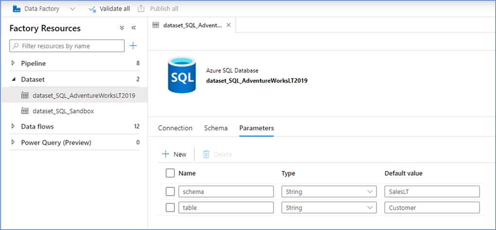
The source component connects to an Azure SQL database that contains the AdventureWorks sample. For this connection a generic Dataset is used, and the schema and table details to connect to are set at pipeline level.

What this means is that a Dataset is defined in Azure Data Factory with its own parameters, so that these parameters can be set for source transformations in the Mapping Data Flow. The screenshot below shows these parameters for the Dataset object, which is independent from where they are used such as in an ADF pipeline or Mapping Data Flow.

Now that the Dataset is available, it can be used for the source connection in the Mapping Data Flow:

The parameters for the Dataset are not visible in the Mapping Data Flow, but they are accessible through the Execute Pipeline that calls the Mapping Data Flow. This is where the values from the JSON file can be assigned to set the connection details.

Technically, this is done by setting pipeline parameters to override the Dataset parameter value with the value from the corresponding JSON segment. The screenshot below shows this. The ‘schema’ and ‘table’ parameters are the ones defined for the Data set, and their values will be replaced by the JSON values and consequently used by the source connection in the Mapping Data Flow.

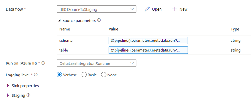
The schema and table values correspond to the following pipeline parameters, which are the names of the properties in the JSON file:

@pipeline().parameters.metadata.runProcessStg.sourceDataObjectContainer
@pipeline().parameters.metadata.runProcessStg.sourceDataObjectDirectory

This approach of using a single Dataset as a generic object by passing in values is but one way to implement a dynamic connection. Some of the other options are using these parameters as dynamic content in the query input or defining an inline source with a similar configuration.

I have opted to use a single dynamic Dataset for the source connection to show how this can be done, and also because a Linked Service to the database is required anyway for Azure Data Factory. But if desired, this can be implement without needing a Dataset at all by using inline connections.

Since the source connection information (schema and table, via the Dataset) is now available, all data from this source can be accessed in the Mapping Data Flow. However, a schema or structure is not defined. There are no columns imported, entered or otherwise defined for now.

Whatever data exists for the connection is now available in the Mapping Data Flow.

The dynamic Derived Column transformation

The Derived Column transformation is really where the templating magic happens. This transformation adds dynamically defined framework attributes to the data that is received from the source. In other words, the data flow contains the data that the connection exposes and adds columns that are defined by the JSON input metadata.

This is achieved using column patterns.

Consider the screenshot below. Three columns are added to the data flow, but their names and values are dynamic – with the exception of the currentTimeStamp(), but this is by design. The $ in the names and values refer to the parameters that are defined for the Mapping Data Flow.

In the previous post, we saw how the JSON design metadata can be configured to populate the parameters at Mapping Data Flow level. These values will now be used to dynamically define the columns and values that will be added to the data flow.

Taking the first column from the above screenshot as an example. When the position equals ‘1’, a column is added to the data with the name of $ldtsAttributeName and expression currentTimeStamp().

The position==1 expression is a trick to make sure the column is added once and only once. The criterion is that if a column exists with (ordinal) position 1, the expression is applied. In other words, if there is data to begin with.

The $ldtsAttributeName parameter contains the intended name of the Load Date / Timestamp column. Looking at the JSON metadata, this column value is ‘LoadDateTimeStamp’.

"ldtsAttributeName": "LoadDateTimeStamp"

The currentTimeStamp() is an expression that is natively available in Mapping Data Flows, and just returns the timestamp of the moment it is called.

This is an example of how columns can dynamically be added using the JSON design metadata. Any value that is passed down for the ldtsAttributeName property will be added as a column in the dataflow with the currentTimeStamp() expression.

The same applies for the second column; $recordSourceAttributeName. In this case, the name is again taken from the parameter but in this example the value is also a parameter. This means that a column with the provided name and value will be added to the data.

"recordSourceAttributeName": "RecordSource",
"recordSource": "adventureworks" 

The last example column that is added in the Derived Column transformation shows a more complex operation; deriving a full row checksum for across the (values of) the provided list of columns.

Using the list of column names, a concatenated string is returned containing the values for each column per row including a sanding element / string concatenator. This can also be implemented as a hash value, in which case a hashing algorithm (e.g. SHA, MD5) can be added to the expression.

For now, showing the values before hashing demonstrates the process more clearly.

To achieve this, the values in the dataItems array from the JSON are parsed into a single value (including sanding elements) and added to the data as a column with the parameter value stored in $rowHashAttributeName.

"rowHashAttributeName": "RowHash",
"dataItems": [
   "CustomerID",
   "NameStyle",
   "Title",
   "FirstName",
   "MiddleName",
   "LastName",
   "Suffix",
   "CompanyName",
   "SalesPerson",
   "EmailAddress",
   "Phone",
   "PasswordHash",
   "PasswordSalt",
   "rowguid",
   "ModifiedDate"
]

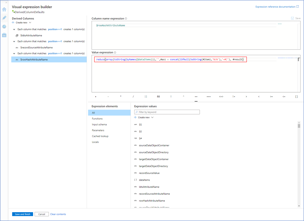
This Mapping Data Flow expression iterates over the array of data items and builds this into a single string value – adding a sanding element for each value. Because the end result is a string value, each individual value is converted to a string with some NULL handling applied.

Interlude – debugging

At this stage we can actually start looking at the data how this is represented through the transformations that already have been configured.

Even though we can’t specify a JSON metadata object at the Mapping Data Flow level, we can still enable the data flow debug feature. What happens is that the default values for all involved parameters will be used, including the defaults for the Dataset parameters. This way, we can still connect the source database as well as look at how the dynamic transformations are applied.

Running the data preview for the Derived Column transformation yields the following results:

The screenshot shown above shows the data as it connects to the AdventureWorks ‘Customer’ table, selects the columns found there and adds the three dynamic columns ‘LoadDateTimeStamp’, ‘RecordSource’ and ‘RowHash’ as per the parameter values.

In the RowHash column, you can see part of the string value that contains the concatenation of the columns that were specified. The ‘~#|’ value is the chosen sanding element. From here, creating a hash value is an easy next step if required.

The (not so dynamic) Surrogate Key transformation

The Surrogate Key really only exists to implement the Source Row Id concept, to generate a incremental integer value for each row in the data set that is processed. The Source Row Id can be added for uniquefication purposes and to cement deterministic behaviour into the data solution, for example when the (high precision of the) effective timestamp is not enough to make each record unique.

In general terms, and in my personal opinion, it is important to implement the Source Row Id concept into a data solution but regardless of this there is another reason why this has been added. The Surrogate Key does not allow a dynamic, paramaterised, name of the created column (key column).

This makes the Surrogate Key transformation somewhat less of a transformation that lends itself to templating.

Or does it?

While we cannot use a parameter to specify the name of the column here, we can define a generic placeholder name in the template. Later on, this placeholder name can be resolved to the intended target name of the Source Row Id column.

For clarity, this should be ‘SourceRowId’ as below – but we will solve this later in the Select transformation.

"sourceRowIdAttributeName": "SourceRowId"

The Select transformation

This source-to-staging pattern is a relatively simple example, so that we can keep focus on the mechanics of creating dynamic and templated data logistics processes. But even in such a simple example a Select transformation is necessary, as it also will be for many of the more complicated templates we will see later.

The Select transformation is used to specify the columns you want to use in the data flow going forward by name, so that you don’t see columns that have served their purpose anymore. This is very helpful in cases when lookups, joins etc. are involved.

Usually, not all column values from all incoming data streams are required to be loaded. It can make sense to make a selection of the columns that are really needed.

We can also use the Select transformation to define dynamic columns even when some transformations do not support this, such as is the case for the Surrogate Key transformation covered earlier. In situations such as these, a generic placeholder name can be covered into the designated name using the parameter value.

This is what happens in the screenshot below.

The ‘name == <>’ expression resolves the name of the column if it exists in the data flow, so this can be made dynamic with parameters. The alias, or ‘name as’ expression also excepts parameters so this is an effective way to only select the columns you need without having hard-coded column names in the template.

More elaborate is the mechanism to cast the names of the dataItems array into individual columns. There is no concept of ‘schema’ so all columns are evaluated whether they have been specified in the array. If they exist there, they will be added.

To my knowledge, unfortunately there is no way to iterate over the array and create a column for each element. In lieu of this it is possible to create a large number of placeholders – one for each position in the array.

This works, because if there are no value for a specific array position the column will simply not be resolved and therefore not added to the dataflow. There will not be a null reference or index issue, the column will just not exist.

In other words, if there are ten columns specified in the dataItems array only the first ten dataItems will result in a column that is stored in the sink.

Obviously, it is necessary to add a lot of placeholder columns to accommodate wide data sets but Mapping Data Flows seems generous on the number of columns that can be added.

The result, when debugging looks like below:

The Sink

Last, but not least, the data is written to the target connection – the Sink. This transformation writes the columns that are available in the data flow at this point to the designated target. The exact columns were already specified by the Select transformation in the previous step, so anything that is defined there will be saved to the target.

The Sink in this example does not use a Dataset object to manage connectivity. It is an example of an inline dataset, as introduced in the previous post. Because of this it is possible to use the target related parameters to define the target connection at runtime.

The following parameters are available for this:

"targetDataObjectContainer": "staging",
"targetDataObjectDirectory": "Customer",

And how they are used:

While this is not visible on the screenshot, except for the icon before the Sink name, the selected connection type is a Delta Lake connection. This template loads data from a database, adds the framework attributes and saves the data into parquet files on the Data Lake that is configured for Delta Lake storage.

It is equally possible to write to any other target that is supported by Azure, but Delta Lake is especially intriguing. It’s a great test case.

The data that is ultimately written (in parquet format) is visible on the Data Lake storage account. A directory will be created following the parameters specified for the Sink if it does not already exists.

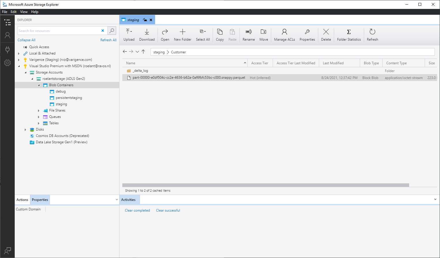
And we can peek in the file from there:

The Data Lake directory acts somewhat as a database table for Delta Lake (with some additional features). It can be used as a source for next steps, which I plan to cover in the next post(s).

We can replicate this process, and create any number of staging Delta Lake directories / tables as long as we provide the design metadata in the designated JSON format.

Of course, the JSON structure used in this series is only one way to organise your metadata. Any (syntactically correct) JSON structure will work, as long as you refer to the property names correctly in the pipeline parameters.

For larger projects, these metadata JSON files can also be stored in a file location that is centrally accessible and the batch process can be configured to load the file from there. It’s very flexible.

Wrapping up the first template

I mentioned earlier that this example source-to-staging template is relatively simple. It is meant to demonstrate the concepts supporting the creation of a dynamic Mapping Data Flow template.

It is created once, but can be run (in parallel) as many times as it is ‘fed’ design metadata.

In the next posts we will look into more complex templates, and consider what it means to produce the JSON files in the first place.

After all, the design metadata has to be codified somewhere.